Perpendicular Parking Robot
VIDEO
A working video demonstration of the robot in action –
Problem Description
The topic of my summer project was to create an autonomous perpendicular parking robot. The robot was a toy car with a non-differential drive steering mechanism. I used three IR sensors, one placed in the rear, one on the right side and one on the left corner to effectively judge the distance between the robot and the side walls or side cars. The car used a simple algorithm using finite state machines to park into its spot effectively. I also placed an LCD on top of the robot for ease during debugging and to display various messages, like “Parked Successfully” after the desired parking has been achieved.
Idea
During a TV show on cars on National Geographic, I saw that certain luxury car owners were privileged with the additional facility of an automated parking system which allowed the driver to sit in the car with their feet on the pedals and press a button to park the car. It was very appealing to me at that time. Later on, when I was browsing through YouTube regarding automated parking techniques I found that there were many models which simulated a parking technique made by students of different colleges. So, I came up with the idea of creating an automated parking robot. Almost all of the parking manoeuvres were for parking the car in parallel. So, I decided to make an autonomous “perpendicular” parking robot.
Parts/Components Used
- ATMEL ATMega32 microcontroller
- L293D Dual H-Bridge motor driver
- NE555 timer IC
- 16 × 2 character LCD display
- 3 × Sharp GP2D120 distance measurement sensors
- NIKKO RC buggy
- Vero boards
- Assorted resistors, capacitors, connectors, transistors
- 220V AC to 12V DC 500mA wall adapter
High level schematic
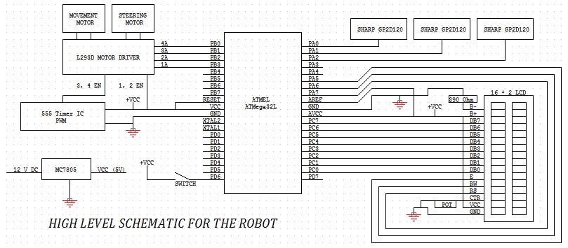
The MC7805 was used to limit the voltage to 5V from the 12V input from the AC wall adaptor. A filter capacitor of 2200uF was used to filter the circuit. The ATMEL ATMega32 was connected to the 5V supply after using a decoupling capacitor of 22pF. The LCD was connected to the right side of the MCU to Port C (data transfer lines) and Port A (selection lines). Port D was used to control the Motor Driver inputs (1A, 2A, 3A and 4A). The motor driver controlled the movement and the steering motors. The 555 timer IC was used to control the 3, 4 EN input of the motor driver to control the movement motor which reduced the speed to a 3/10th. The 3 analog inputs from the SHARP GP2D120s was interfaced with the Port A ADCs.
Proposed Solution Model
Part A: Parking algorithm using a finite state automata
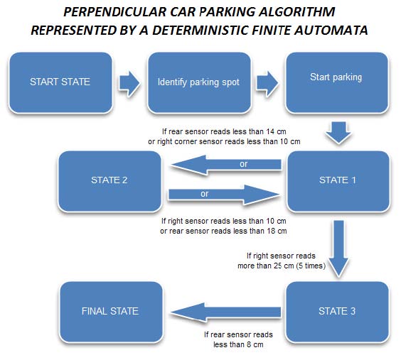
As can be seen in the block representation, there are three main states which determine the parking orientation. Initially, the robot is in the start state. Then it moves straight forward until it identifies the parking space. This is done by the sensor readings from the sensor on the right. After it identifies the parking space it goes to the Start parking state.
The details of the three important parking states as shown in the DFA by 1, 2 and 3 are given below.
- State 1:
The robot wheels are turned right and the robot starts moving backwards. If the rear sensor reading is greater than 14 cm, then the robot remains in this state. When the rear sensor reads some value less than 14 cm, then the robot goes to State 2. If the right sensor reads more than 25 cm, then the car will continue changing between states 1 and 2 for five times ONLY (this is to ensure that the car aligns itself properly w.r.t the parking spot. If the left corner sensor reads less than 10 cm, the car goes to state 2.
- State 2:
The robot wheels are turned to the left and the robot starts moving forwards. If the rear sensor reading is less than 18 cm, then the robot remains in this state. When the rear sensor reads some value greater than 18 cm, then the robot goes to State 1 again. Again, if the sensor on the right reads a value greater than 10 cm, then also the robot goes to State 1 again (this is to ensure that there is not a lot of space left on the right side of the car).
- State 3:
This is the state the robot reaches when it has entered the parking spot. When this state is reached, the robot aligns its wheels straight and starts backing until the rear sensor reads less than 8 cm. So, effectively the robot gets parked at a distance of 6-8 cm from the rear end.
NOTE: This algorithm has been found to work with this model of toy car only. So, the algorithm values will vary if a different car is used to test this algorithm. The values used in the algorithm have been found out after testing the motion of the car rigorously. The robot had a non differential drive steering mechanism which made it difficult for the robot to make sharp turns which in turn caused the inadvertent thrashing of wheels from left to right to align itself to the side walls.
Part B: Pseudo code for the autonomous car parking algorithm
  LOOP identify_spot(right_s, identified = 0)
  begin
       if (!identified)
       begin
           if (right_s > 10 cm)
           begin
               identified = 1
               continue
           end
           if ((identified = 1) AND (right_s < 10))
           begin
               identified = 2
               goto parking
           end
       end
  end

  LOOP parking(rear_s, right_s, lcorner_s, parked = 0, state = 1)
  begin
       if (NOT parked)
       begin
           if (state = 1)
           begin
               all_stop()
               turn_right()
               move_backward()
               if (rear_s < 14 cm)
                   state = 2;
               if (right_s > 25 cm)
               begin
                   align_count = align_count + 1;
                   state = 2;
                   if (align_count == 5)
                       state = 3;
               end
               else if (lcorner_s < 10 cm)
                   state = 2;
           end
           if (state = 2)
           begin
               all_stop()
               turn_left()
               move_forward()
               if (rear_s > 18 cm)
                   state = 1;
               if (right_s > 10 cm)
                   state = 1;
           end
           if (state = 3)
           begin
               all_stop()
               move_backward()
               if (rear_s < 8 cm)
                   state = final_state
           end
           if (state = final_state)
           begin
               all_stop()
               LCD_WRITE(“PARKED SUCCESSFULLY”)
               parked = 1
           end
       end
  end
Experimental Results and Discussions
The first hurdle was to create a proper driver software for the MCU to effectively communicate with the LCD. So, the HD44780 driver datasheet was referred and created the software driver to run in the 8-bit communication mode with 5 * 8 char display. After the LCD had been properly interfaced with the MCU, the SHARP GP2D120 distance measurement sensors had to be interfaced with it. So, 25 different ADC readings were taken off the MCU and a plot of the ADC values with its corresponding distance values was made.
Initial sensor readings:
| ADC values | Distance |
| DIFFICULT TO RESOLVE | 1 cm |
| DIFFICULT TO RESOLVE | 2 cm |
| 615 – 620 | 3 cm |
| 574 – 579 | 4 cm |
| 485 – 490 | 5 cm |
| 418-422 | 6 cm |
| 365-369 | 7 cm |
| 322-327 | 8 cm |
| 289-294 | 9 cm |
| 260-264 | 10 cm |
| 233-238 | 11 cm |
| 214-219 | 12 cm |
| 198-202 | 13 cm |
| 188-193 | 14 cm |
| 177-182 | 15 cm |
| 166-170 | 16 cm |
| 157-160 | 17 cm |
| 147-150 | 18 cm |
| 139-142 | 19 cm |
| 129-132 | 20 cm |
| 122-125 | 21 cm |
| 117-120 | 22 cm |
| 109-113 | 23 cm |
| 106-109 | 24 cm |
| 102-104 | 25 cm |
| < 102 | > 25 cm |
The plot resembled very much with the one given in the datasheet for the SHARP sensor which was very satisfactory.
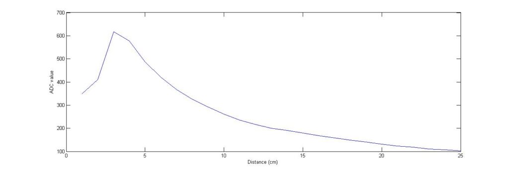
As can be seen, the graph is not linear and it was not possible to develop an effective yet simple equation for this graph. So, a normalization was needed which was essentially linearization in this case.
Linearized/Normalized sensor readings
| Distance | ADC value | 1 / Distance |
| 4 cm | 577 | 0.250 |
| 5 cm | 487 | 0.200 |
| 6 cm | 420 | 0.167 |
| 7 cm | 367 | 0.143 |
| 8 cm | 325 | 0.125 |
| 9 cm | 291 | 0.111 |
| 10 cm | 262 | 0.100 |
| 11 cm | 235 | 0.091 |
| 12 cm | 217 | 0.083 |
| 13 cm | 200 | 0.077 |
| 14 cm | 191 | 0.071 |
| 15 cm | 179 | 0.067 |
| 16 cm | 168 | 0.063 |
| 17 cm | 158 | 0.059 |
| 18 cm | 149 | 0.056 |
| 19 cm | 141 | 0.053 |
| 20 cm | 131 | 0.050 |
| 21 cm | 123 | 0.048 |
| 22 cm | 118 | 0.045 |
| 23 cm | 111 | 0.043 |
| 24 cm | 107 | 0.042 |
| 25 cm | 103 | 0.040 |
The normalization was performed by taking the reciprocal of the distance and then taking a plot of the inverse distance versus ADC value. This gave a fairly linear plot which was more usable than the earlier graph. After the normalization was performed, the graph had two major changes in the slope at ADC values 205 and 577. So, the graph was divided into three line segments with a fairly consistent slope. But later on, the second line segment had to be divided into two line segments because the distance readings that were obtained were not very reliable. So, at the end the plot got divided into four different line segments.
The plots showing the initially divided three line segments –
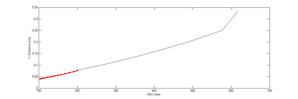
The ADC equation used for the first line segment as shown in Fig 4 is –
For ADC values between 101 – 205,
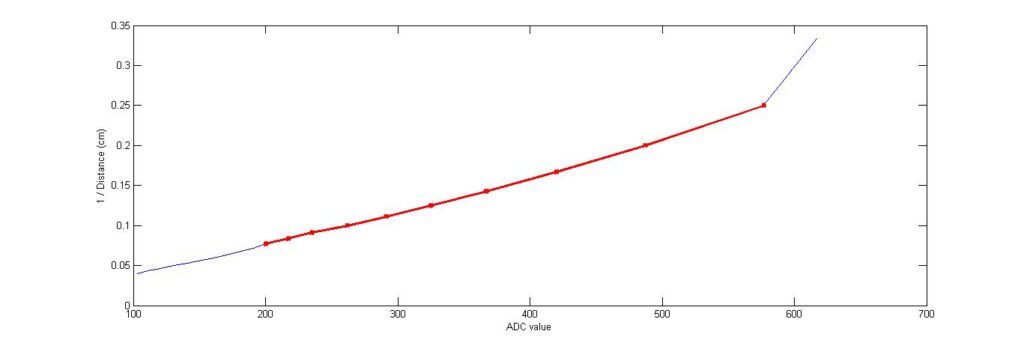
Fig 5. shows the second line segment which seemed to have a fairly consistent slope at first but was found to be inaccurate and unreliable when used with one line equation to find out the distance covered by this segment. So, the line segment was divided into two which gave better results.
The ADC equations for the second line segment(s) are –
- For values between 287 – 577
- For values between 208 – 287
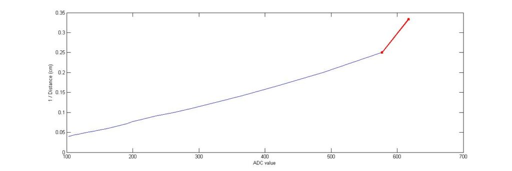
The equation for the third line segment as shown in Fig 6. is –
For ADC values between 577 – 617,
After using these ADC equations to interface the SHARP distance measurement sensor, a fairly accurate distance reading was outputted to the LCD screen. Next task was to solder the circuit on a veroboard which had been bought keeping the dimensions of the toy car in mind. After soldering, the circuit board was mounted on the robot.
Two buffers were used to amplify the signals from the MCU to the motor driver pins controlling the movement motor.
Next was to use a speed which allowed sufficient time to the MCU to properly be able to process the distance readings and use the correct states. I decided to use an external PWM because I had already soldered the motor driver pins and MCU pins. So, I decided to use a 555 timer IC to generate the pulses. Initially, a duty cycle of 1/10 was set for the motor but it rendered the robot motionless. Later, a 3/10 duty cycle was found out to be effective in controlling the motor speed.
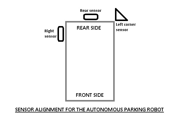
Then the algorithm was implemented and debugged. The sensors were aligned in a manner such that all the sensors would be involved and none would be rendered idle while parking.
Conclusion
The results obtained by using the sensors in this manner were overwhelming. The car parked with a fair degree of accuracy. The various perks of this model are discussed below.
The major limitation of this model is that it does not align itself exactly parallel to the side cars (or walls, in this case made of white thermocol sheets). And because of this, during some trial runs, the car hit the side wall inside the parking space while backing straight up. This problem did not arise in the initial algorithm testing stage but while demonstrating the car’s ability using the same algorithm; it was found that the algorithm lacked a certain degree of usability chiefly because of the inaccuracies related to the sensor readings. So, the alignments of the sensors were changed and the algorithm was modified for better adaptability in various lighting conditions.
Also, the car needs to be placed at a certain distance of about 3 cm from the side of the wall to attain the most desirable parking result.
Lastly, the algorithm won’t work in case there is no closed space for parking, i.e. it can only park between two walls and not alongside one wall.
Nevertheless, this algorithm is fairly accurate. The ambient lighting conditions should not be very bright so as to swamp and interfere with the sensors and the walls should be preferably white for high reflectivity.
The car is able to identify the spot and get into it, but sometimes the alignment of the car to the side cars is not straight and because of this, 1 out of about 7 times, it tends to hit the side wall while backing up. This was not the case with the initial algorithm because it was based on the exact conditions of the room where the testing was performed and the algorithm didn’t look very adaptable. But this algorithm can work in a variety of lighting conditions with a fair amount of accuracy.
I would definitely say that this algorithm is very reliable given the constraints of ambient light and the inaccuracy of the Sharp distance sensors.
So, I would like to conclude by stating that I am deeply satisfied with what I have been able to achieve in the past couple of weeks and that the end result was very satisfactory.
References
Books
- Designing Embedded Hardware – O’Reilly – John Catsoulis
- Electronics for Dummies – Gordon McComb and Earl Boysen
Web references:
- Robozeal Blogspot LCD interfacing
- AVR Fuses Guide
- Linearizing Sensor readings guide
- AVR Freaks
- Programming AVR Fuse Bits at ScienceProg
Datasheets: