Nonlinear optimization using LM
July 15, 2023
This is a tutorial on how to perform nonlinear least squares in Python using scipy.optimize.least_squares. The reader is expected to know about linear and non linear least squares and the kind of problems they are used to solve.
In this tutorial, we are going to take an example of a function  .
.
Given observed values  , and values of
  , we would like to estimate the parameters
  for the function
  where when we plug in the values of and
  , we should get
  close to .
We are going to use observed values that were created using a value of 2. And then in the code, we add some noise to this in the function add_noise_to_observed_values.
Result
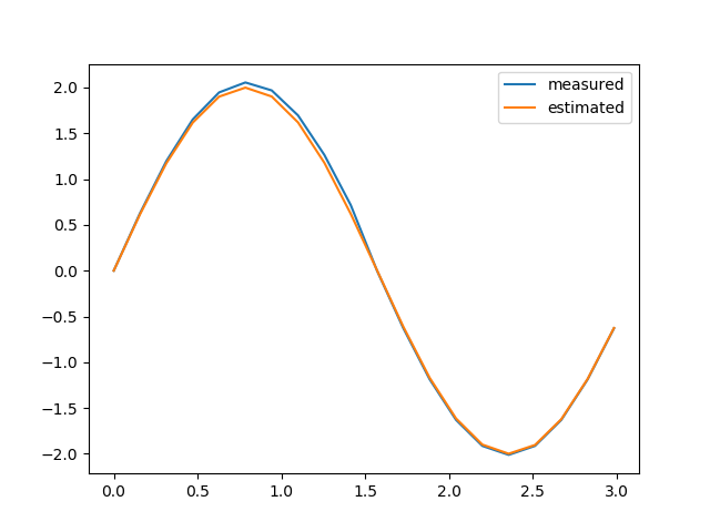
y_obs and y_est values.Python Code
# y = f(x, v) = v * sin(v * x)
# where, x = input values
#        v = parameter values that needs to be estimated
#        y = output values
#
# Given observed values of y, and values of x, we would like to estimate the
# parameters 'v' for the function f(x, v) where when we plug in the values of
# 'x' and estimated 'v', we should get 'est_y' close to 'y'.
#
# @note: We need to know the function signature, or atleast have access to
#        a blackbox function call that takes in (x, v) as arguments and gives
#        us 'y'.

import numpy as np
import matplotlib.pyplot as plt
import math

from scipy.optimize import least_squares

def fn(x, v):
    '''
    Given 'x' and 'v', estimate the function output, i.e. the 'y' value.
    '''
    fn = v * math.sin(x * v)
    return fn

def fn_residual(v, x, y_measured):
    '''
    Residual = y(x, v) - observed_value_of_y

    For every element in 'x', and corresponding element in 'y_measured',
    calculate the residual between fn(x[i], v) and y_measured[i].
    '''
    residuals = []
    for i in range(0, len(x)):
        residual = fn(x[i], v) - y_measured[i]
        residuals.append(residual)

    return np.array(residuals).flatten()

def plot_measured_and_estimated_fn_values(x, y, est_y):
    '''
    Plot 'y' and 'est_y' to visually inspect the quality of the nonlinear fit
    '''
    plt.plot(x, y, label='measured')
    plt.plot(x, est_y, label='estimated')
    plt.legend()
    plt.show()

def add_noise_to_observed_values(obs_y):
    '''
    Add some noise to the observed values
    '''
    for i in range(0, len(obs_y)):
        if i < len(obs_y) / 2:
            obs_y[i] += 0.011 * i
        if i > len(obs_y) / 2:
            obs_y[i] -= 0.011

    return obs_y


def main():
    # Values of 'x'
    x = [(i * math.pi / 20) for i in range(0, 20)]

    # Observed values of 'y' for the given values of 'x'
    # These values were obtained using 'x' and v = 2
    obs_y = np.array([0.0, 0.6180339887498948, 1.1755705045849463, 1.618033988749895, \
                      1.902113032590307, 2.0, 1.9021130325903073, 1.618033988749895, \
                      1.1755705045849465, 0.618033988749895, 2.4492935982947064e-16, \
                      -0.6180339887498955, -1.175570504584946, -1.6180339887498947, \
                      -1.902113032590307, -2.0, -1.9021130325903073, -1.6180339887498951, \
                      -1.1755705045849467, -0.6180339887498953])

    obs_y = add_noise_to_observed_values(obs_y)

    # Levenberg Marquardt (LM) is sensitive to initial values, so choose an initial value
    # as close as you can possibly start off with.
    initial_values = [1]

    # fn_residual takes (v, x, y_measured), where (x, y_measured) remains constant, which are provided
    # in the 'args' parameter.
    least_squares_result = least_squares(fn_residual, args=(x, obs_y), x0=initial_values, method='lm')
    est_v = least_squares_result.x

    est_y = []
    for val in x:
        est_y.append(fn(val, est_v))

    print(F'Estimated value of v: {est_v}')
    plot_measured_and_estimated_fn_values(x, obs_y, est_y)

if __name__ == '__main__':
    main()