Lifelong Mapping in the Wild

For more details about this work, click here for the Elsevier RAS Journal article. Individual sections of this article were published in detail at ICRA (Node Marginalization), IROS (View Management), and ECMR (Adaptive Local Maps, Preventing & Correcting Mistakes in Mapping).

1. Introduction

Household cleaning robots have become common, making up 20% of current vacuum market, and have freed millions of people from mundane chores. These robots map their environments using Simultaneous Localization and Mapping (SLAM) to maximize floor coverage and return to a charging station. More advanced models incorporate semantic knowledge about the environment into their maps. This allows users to direct the robot to clean a particular room or spot on the floor.

One challenge of mapping a “wild” household environment rather than a well controlled research space is that its appearance and structure changes over time. Changes in lighting from day to night alter the visual features a robot’s camera can observe. Moving a couch both alters the appearance of a room and invalidates the robot’s occupancy map. Thus, a static map quickly becomes outdated and useless. On the other hand, creating a new map on every robot run precludes useful behaviors, such as cleaning a specific room. Therefore, our goal is lifelong mapping, in which the robot updates its map continuously to reflect changes in its environment.

We first describe a lifelong mapping system for a robot equipped with a monocular camera. The map created by the system consists of three layers (Fig. 1):

the SLAM system’s model of the environment’s appearance that the robot can use to localize itself, which is the combination of a graph and its views
an occupancy map to model the environment’s structure that the robot can use for path planning accurately
a semantic map to fuse all of the robot’s knowledge in a stable fashion that can be understood and interacted with by an end user

We use the terms SLAM graph, pose graph, and graph largely interchangeably since our implementation is based on a pose graph. However, the methods outlined apply to any graphical SLAM system. The first two layers consist of local-scale elements: views, SLAM graph nodes and edges, and local occupancy maps. As the robot works, it continuously adds new local-scale elements. As these elements grow in number, memory and CPU consumption skyrocket, which starts to have an adverse effect on localization accuracy when memory and/or CPU usage limits are reached. It is therefore imperative to remove redundant and outdated elements from the map without compromising its integrity. To that end, we present a set of algorithms for intelligent pruning of the local-scale elements.

Fig 1: Our lifelong mapping system partitions spatial data into three layers: the SLAM pose graph (left), occupancy map (center), and semantic map (right). The first two layers contain local-scale elements whose growth must be constrained. The semantic layer contains global-scale elements which must be stabilized.

The semantic layer of the map consists of global-scale elements, such as room boundaries, physical objects (e.g. a fridge, a couch) which are commonly understood by the user and the robot. Semantics in the home tend to be stable over time with occasional changes such as adding a new room to the home or moving furniture. We present an approach for consistent maintenance of the semantic layer, thus enabling lifelong map-based interaction between the user and the robot.

We include the following strategies from our previous work for keeping the map complexity stable over time, while allowing it to evolve to adapt to changes in the environment:

View Management (ref)
Pose Graph Simplification (ref)
Pruning of Local Occupancy Maps (ref)

We go into detail about maintaining map accuracy, by covering strategies for ensuring semantic map stability. We also cover the strategies for preventing relocalization and recovery errors, in order to reduce the probability of localizing into the wrong map, or making an erroneous pose correction caused by similarlooking structures in different parts of the environment.

Despite all these measures, the probability of a mapping or localization error occurring is non-zero. With lifelong mapping, there eventually will be times when the error in the robot’s pose estimate is high enough to affect the occupancy map or
the robot’s semantic understanding of the environment. To address the corruption of the occupancy map, we present a method for detecting erroneous protrusions in the map, typically caused by wheel slippage.

We evaluate our system on real robots in realistic scenarios. We show experimental results, demonstrating that the system can adapt to changes in the environment, while keeping the map size stable across multiple runs.

To summarize, our contribution is two fold. First, we present a complete lifelong mapping system by integrating our previous works on ensuring map stability and accuracy with a graph-based monocular SLAM system. Then, we present a large-scale evaluation of the aforementioned lifelong mapping system in 10,000 robots with close to 1 million robot runs across various geographic locations in the world.

2. System Overview

In this section, we describe our overall navigation and mapping system, which consists of a SLAM module, an occupancy map module, and a semantic map module (Fig. 2).

Our lifelong mapping robot is designed around a graph-based monocular visual SLAM system as proposed by Eade et al (ref). The SLAM system takes as its inputs a sequence of images from the camera, and a sequence of differential motion estimates from wheel encoders or other differential sensor, which we simply call odometry. As mentioned before, the SLAM system consists of a front-end and a back-end. The graph representation of the SLAM back-end also serves as
the topological map in a hybrid map occupancy mapping system. Semantics are overlayed on the rendered occupancy map by means of a global meta-semantic layer.

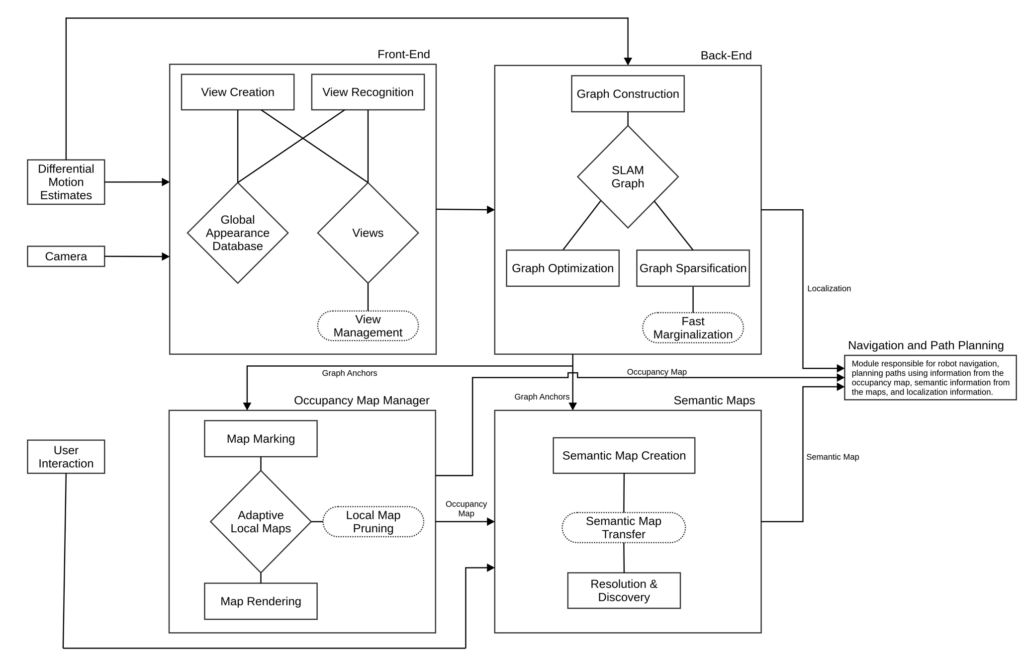
Fig 2: **System architecture.** The system consists of the following modules: SLAM, occupancy map, and semantic map. Each module includes algorithms for its maintenance during lifelong mapping, shown in dotted ovals.

2.1 SLAM : Front-End

The front-end takes images from the monocular camera several times per second as inputs, and performs two operations: view creation and view recognition.

During view creation, the front-end generates a new view, which is a 3D point cloud with associated visual feature descriptors. The point cloud generation is achieved through a structure from motion approach. Each view is associated with a node in the pose graph. If the view is of high quality, it is added to a view database. During view recognition, the front-end observes the previously created views by querying the robot’s view database, and comparing its calculated view to those in the database. If a matching view is present, the front-end estimates the robot’s position and orientation relative to that view and relays this information to the back-end for graph encoding.

2.2 SLAM : Back-End

The back-end maintains a pose graph, whose nodes are robot poses, and whose edges are measurements that encode pairwise constraints between them. Some of the nodes may be associated with other entities, such as the views from the frontend, or local maps described in Section 2.3.

The pose graph contains both motion edges generated by odometry measurements and observation edges generated by the front-end’s observations of views. The observation edges create loop closures in the graph, which provide the constraints necessary to ascertain the maximum likelihood estimate of each pose through a statistical optimization. Specifically, we solve for the time-indexed sequence of robot poses X¹,··· ,X^N which minimize energy functional –

$\sum_{ij} {||\log (X^i (\mu_{ij} X^j)^{-1})||^2}_{\Lambda_{ij}} \chi_{ij}, \quad i \ne j, \; i, j \in {0, 1, \cdots, N}$

where $X^0$ is a constant and $\chi_{ij}$ evaluates to 1 when there is a measurement edge of mean $\mu_{ij}$ and information matrix $\Lambda_{ij}$ from node $i$ to $j$ , and 0 otherwise. Note that the number of nonzero terms in the sum is also the number of edges in the graph.

The above energy functional can be rewritten in terms of the relative poses between nodes –

$\sum_{ij} ||\log (\Delta_{ij} (\mu_{ij})^{-1})||^{2}_{\Lambda_{ij}} \chi_{ij}, \quad i\ne j, \; i,j\in{0, 1, \cdots, N}$

where $\Delta_{ij}=X^i(X^j)^{-1}$ is the relative pose from node $i$ to node $j$ . The pose graph can be optimized by one of the many available incremental graph optimization methods, making sure that computations are bounded.

The size of the pose graph grows over time as the robot explores the environment, so we need to simplify the graph by pruning nodes and edges. The graph simplication is introduced in detail in 3.2.

2.2.1 Hypothesis Filter

When a home robot is kidnapped, it will lose the information of its present location. To cover all cases, the robot can simultaneously build a new pose graph component from scratch and search for views from prior components. We use the term Component to refer to one fully connected graph and the term Graph to denote one or a collection of components that are disjoint. Suppose our robot has mapped a single space as a pose graph component $C_a$ . When it is kidnapped, the robot will create a new, empty component $C_b$ which will be used for localization and mapping. If the robot later observes a view corresponding to a previous observation in $C_a$ , it can localize itself in $C_a$ by adding an edge between its current node in $C_b$ and the node for the previously observed view in $C_a$ . This results in a merge between the connected components.

Unfortunately, a view observation can be incorrect. The front-end can mistake similar-looking features of the environment for each other. Even after observing the correct view, errors in pose estimation can arise from image noise, motion blur, and changes in illumination. Therefore, merging $C_a$ and $C_b$ , based on a single observation is risky. Instead, if the robot observes a view from a prior component, we form a merge hypothesis that the two components should be joined, but delay the actual merging of the components until we accumulate enough evidence for the merge hypothesis.

Similarly, the robot may detect a new view in its current pose graph component which contradicts its current pose estimate. This may result either from an incorrect view observation or from the accumulation of odometry errors. As before, adding an observation edge immediately risks destruction of the map. The robot would be wise to turn the view observation into a recovery hypothesis, and wait to see if more evidence for it presents itself.

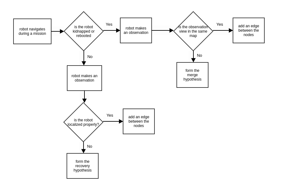
The hypothesis filter (Fig. 3) is our method for managing merge and recovery hypotheses. The hypothesis filter represents each hypothesis as an Extended Kalman Filter (EKF), whose state is updated by robot motion and view observation. We accept a hypothesis by adding edges to the SLAM graph for view observations that support it. For a merge hypothesis, new edges are all between the same two disjoint connected components, whereas for a recovery hypothesis, the edges are all within a single connected component. Acceptance criteria for a hypothesis in our case is based on preset thresholds on the number of view observations contained in the hypothesis and the number of views that were observed. It is also helpful to keep the number of hypotheses from becoming too many and we keep this from happening by imposing expiration criteria.

2.3 Occupancy Mapping

Our occupancy maps are based on the adaptive local mapping system (ref1, ref2). Instead of a single global occupancy map, we use a collection of overlapping local maps, which are anchored to nodes in the pose graph described in Section 2.2. The local maps move together with their respective nodes, when the graph is optimized. This automatically incorporates the most up-to-date pose estimates into the occupancy map. When we need to plan the robot’s path, we collapse the current configuration of the local maps into a single global occupancy map – an operation we call rendering.

2.4 Semantic Mapping

Our semantic mapping layer is the interface between the user and the robot. It is also used by the robot for coverage planning. The semantics are high level concepts, extracted from the other layers in the system, that both the user and
robot understand. Examples include rooms (sub-area representing a room in the house), walls (exterior and interior boundaries of static objects, such as real walls), clutter (dynamic objects that can be filtered out of the map) and dividers (separation that splits different rooms in the house, such as doors). The semantics also have relative constraints between them in order to guarantee their validity. For instance, dividers are constrained to end on walls so that they partition the map into disjoint rooms. Our system makes use of both automatic algorithms as well as optional user annotation that they provide through an app to determine the semantics. The semantic map allows intuitive user experiences, for example, the
ability to have the robot clean a particular room everyday, or clean the rooms in a predetermined order. It is hence important to guarantee that the semantic map stays consistent with the robot representation of the environment for the life time of the robot.

3. Lifelong Mapping: Maintaining System Performance

In this section, we first discuss the strategies for maintaining system performance by reducing map complexity over time. At the end of this section, we present experimental results and a short discussion on the performance of these strategies.

3.1 View Management (More details)

There is a trade-off fundamental to the SLAM front end’s aggregation of views during lifelong mapping (Fig. 4). Generally, each new view increases the chance that the robot will successfully correct its pose or relocalize at a later time. On the other hand, an increasing large library of views consumes extra memory and requires more expensive searches during relocalization, even when accelerated with smart search data structures. Furthermore, during the lifetime of a robot, changes to the environment will often invalidate views or render them obsolete. As a result, some views are more useful, available, and informative than others. These views are usually the ones that are more agnostic to lighting or environmental
changes, and are observed more often.

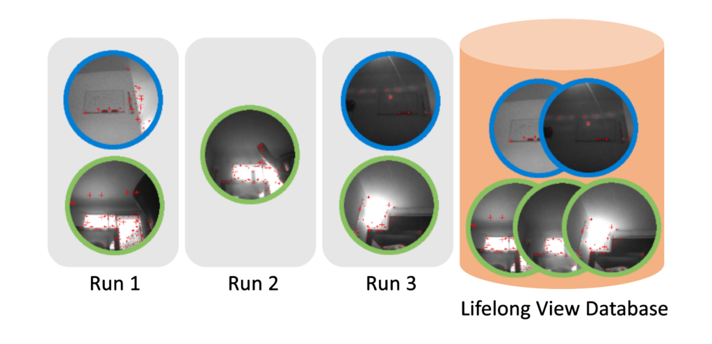
Fig 4: Aggregation of generated views of the same scene from different times of day in a household environment to aid in lifelong mapping. More and more views consume more memory and require expensive searches during observation and relocalization.

Our solution to controlling the growth of views in the front end is simply to delete them. However, we must be careful to delete only those views which are unlikely to be useful in the future. We do so with a constrained energy minimization procedure that optimizes the trade-off between sparsity and probability of relocalization. Our method scores existing views with a utility function composed of short-term and long-term observation statistics. The front end then removes each view with a low score if and only if there are other views nearby to which the robot could localize to instead of the one to be pruned. As a result, poor-quality and outdated views are pruned, but no one region of the mapping environment loses its respective views altogether.

3.2 Graph Simplification (More details)

Keeping computation time for graph optimization manageable is a challenge for lifelong mapping. The graph represents the information the system has gained over time about the environment. More information is being added to the graph
all the time as the robot receives incremental motion information from its various sensors. Thus, the complexity of the graph grows, increasing the cost of optimizing it. To counteract the additional information being added, the lifelong mapping solution must reduce the graph complexity periodically while preserving as much information as possible.

Our approach to graph simplification is based on two operations. We occasionally remove edges that are the least informative to limit the total number of edges in the graph to be proportional to the number of nodes. We also occasionally
remove nodes from the graph using a fast marginalization method, provided those nodes are not associated with any other entity, like a view or a local map.

The marginalization replaces the sub-graph consisting of the node to be removed and the edges to its neighbors with new edges between the neighboring nodes of the node being removed. Our approach uses a nearly optimal approximation of the marginal distribution with the target node removed that can be computed extremely quickly even on limited hardware resources. Specifically, our method is based on defining a target topology for simplified graph and then performing a weighted average over all possible tree based approximations that land on the target topology.

3.3 Pruning of Local Maps (More details)

In a lifelong mapping scenario, new local maps are continuously generated. Without pruning, their number will grow without bound (Fig. 5), overflowing the memory constraints of the system and making the cost of rendering the global map unacceptable.

Fig 5: Not having pruning in a lifelong mapping scenario results in an overgrowth of redundant local maps (right) over time, increasing memory and CPU consumption.

Choosing a subset of local maps to prune is tantamount to destroying information – a questionable maneuver in a field where more data generally provides higher accuracy. While pruning local maps reduces memory consumption, it may also deteriorate the global map we generate from these sub-maps. Our goal then is to limit this deterioration. This insight allows us to formalize local map pruning as the constrained optimization problem –

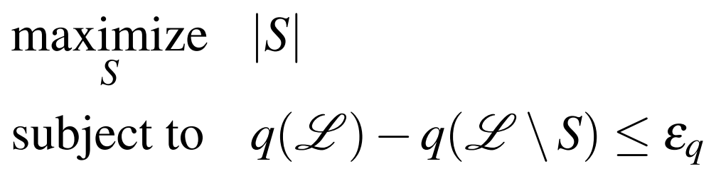
where $\mathcal{L}$ denotes the set of all local maps, $S$ denotes the subset of these to be deleted, $q$ is a metric which scores the result of rendering a global map from a given subset of maps, and $\epsilon_q$ is a tunable parameter for the allowable deterioration of the rendered map.

The above expression is clearly too general to solve directly for a global optimum. To illustrate, if $q$ were chosen to count the number of nodes in the underlying pose graph which were not adjacent to any local map pose nodes, and $\epsilon_q$ were chosen to be 0, the global optimum would be the complement of the minimum vertex cover for the pose graph. Instead we rely on a greedy optimization which adds local maps to $S$ in an order determined by a heuristic cost function. After each addition to $S$ , we verify that $\mathcal{L} - q(\mathcal{L} \setminus S) \leq \epsilon_q$ . If our inequality does not hold, we remove the new local map from $S$ .

3.4 Experiments and Results

3.4.1 Data Set

We collected map metrics and mission (a robot run) statistics from a fleet of robots deployed in real-world indoor environments. No images from the robots were ever viewed, nor were they ever stored or processed off of the robot. From our fleet, we selected 10,000 robots running in different geographic locations all over the world; specifically, we chose those robots with the longest lifespans, up to 200 consecutive runs per robot. This subset was chosen to maximize the
opportunity for lifelong mapping failure modes to occur. In total, the data set contained data from 965,561 runs over a period of six months. We call this dataset – Dataset A.

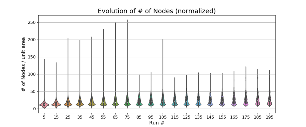
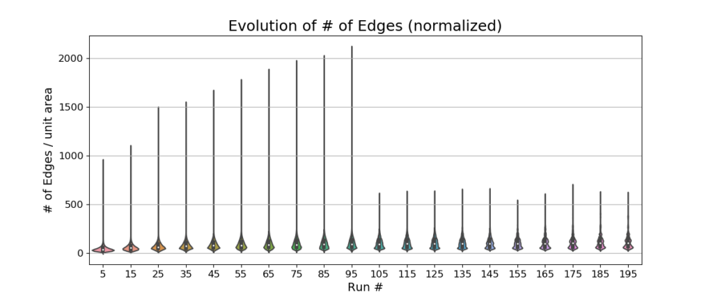
3.4.2 Map Growth Metrics

For evaluating the growth of the map across robot runs we simply count the number of the local-scale elements of the map: nodes, edges, views, and local occupancy maps. We also calculate the total size of the map on disk.

3.4.3 Evaluation

Fig. 6, Fig. 7, and Fig. 8 show the evolution of maps on 10,000 robots running in consumers’ homes as violin plots. These plots depict distributions of the normalized data per unit area or scaled data across run / mission number (i.e., the number of sequential runs on a particular map with continuous updates) groups using density curves. The unit area used is arbitrary, but could be, for example, a square meter. The width of each curve corresponds with the approximate frequency of data points in each region. The evolution of the total number of nodes and edges (normalized per unit area) show that the SLAM graph memory consumption remains stable over time due to the graph simplification operations. The sudden shortening of the tails of the number of edges between 95 and 105 missions is related to a small number of robots in our dataset that have run fewer than 100 missions. The increase in tail length for the number of nodes around 105 missions is an outlier which doesn’t affect stability.

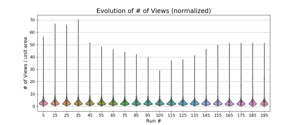
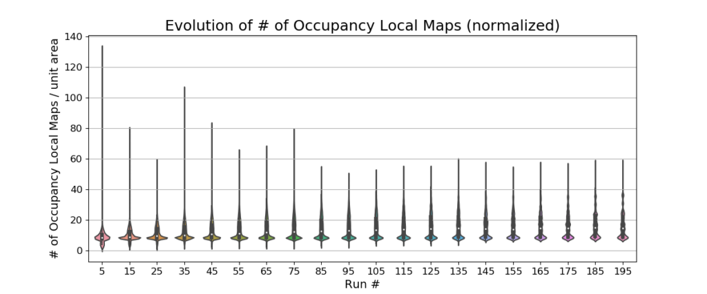
Fig 6: Evolution of the number of nodes and edges in Dataset A. The nodes and edges remain stable across 200 robot missions. The X-axis denotes the run/mission number, and the Y-axis denotes the number of nodes and edges per unit area.

Fig 7: Evolution of the number of views and local maps in Dataset A. The views and local maps remain stable across 200 robot missions. The X-axis denotes the run/mission number, and the Y-axis denotes the views and local maps per unit area.

There is also no observable change in the number of views (per square meter) or the number of adaptive local maps across 200 runs. This indicates that the view and local map pruning algorithms have stabilized the number of views and local maps.

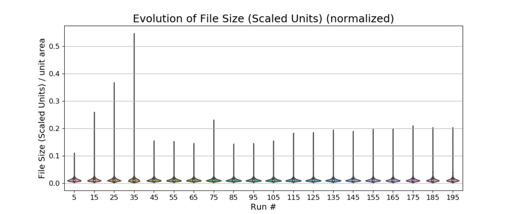
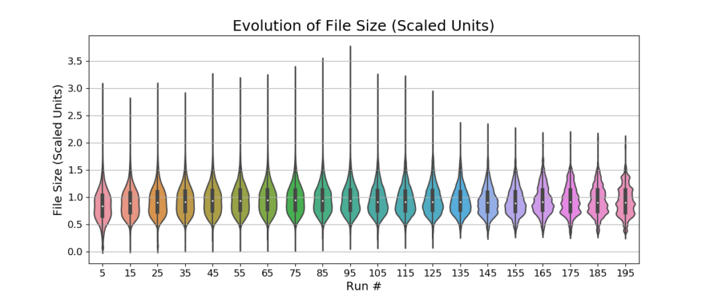
Fig 8: Evolution of map file size in Dataset A. Map file size remains stable across 200 robot missions. The X-axis denotes the run/mission number, and the Y-axis denotes the map size in scaled units, both normalized (per unit area) and raw.

The overall map size on disk does not change significantly across runs. This means that the proposed algorithms working together keep the map stable in terms of memory consumption.

4. Lifelong Mapping: Maintaining Map Accuracy

In this section, we cover strategies that ensure semantic map stability, methods to prevent relocalization and recovery errors, and to detect erroneous protrusions in occupancy maps. Finally, we present experimental results and discuss the performance of these methods.

4.1 Adaptive Semantic Mapping

As previously described, semantics consist of high level concepts such as walls, rooms, dividers, and clutter, as well as relative constraints between these concepts. The challenges of noisy sensing, localization uncertainty, dynamic objects and large changes in the environment, need to be addressed in the context of semantic maps. This will guarantee consistent smart behavior for the lifetime of the robot.

We represent the semantics as polygons and segments on the 2D floorplan. It is natural to expect the system to track and evolve these semantics over time. We achieve this by leveraging the SLAM framework which allows one to associate real world coordinates to the 2D floorplan locations of the semantics. By anchoring the points to the SLAM framework, we rely on the robot’s localization system to track the locations of the semantics over time. This approach has limitations, particularly due to the uncertainty in the localization system and dynamic obstacles. Further, the constraints between semantics can get violated if we rely solely on the localization system’s tracking of points. For instance, we constrain the wall semantic to lie close to an occupied pixel sensed by the robot in order to guarantee tight coverage of the home. Tracking wall segments through SLAM alone does not guarantee this constraint over time. Hence we use the tracked locations to transfer some semantics and recompute other semantics based on the underlying occupancy map and the transferred semantics. The reader is referred to (ref) for details. Briefly, we use SLAM based tracking to classify wall and clutter pixels in the occupancy map. We recompute the wall semantic from the classified occupancy map. Using the tracked divider end-points and by reprojecting them to the nearest wall pixel, we are able to reconstruct all the semantics from the previous map in the new one. We call this process semantic map transfer.

Despite semantic map transfer, occasionally inconsistencies occur in the semantic map. Inconsistencies such as loss of a room or divider are automatically detected and resolved using a module for conflict detection and resolution. For instance, we detect disconnected walls which were connected in the previous map. Then, through geometry processing of the difference between the anchored room boundaries and the new walls, we recover the original connected topology of the walls in the new map.

Finally, a dedicated discovery module is responsible for adding semantically meaningful changes as they are detected. For instance, if a new space is explored in the home, automatic room discovery algorithms are triggered to handle the addition of the space as a new room to the map.

Our system is thus able to account for true changes in the environment, such as addition of new rooms to the home and moving of large pieces of furniture. This is accomplished without losing semantics due to noise and small dynamic objects. For a detailed explanation of this process, see (ref).

4.2 Preventing Incorrect Relocalization

Acceptance criteria for a merge hypothesis present a trade-off. If they are too permissive, the robot may localize into a wrong component, or it may localize into the right component, but in the wrong place. If the acceptance criteria are too
strict, then the robot may take a long time to localize, during which it will not be able to perform many tasks, such as navigating to a specific room.

We propose to get the best of both worlds by having two sets of acceptance criteria: a permissive set for a conditional merge of the two components, which can be undone, and a strict set for a full merge, which cannot be undone. The idea is for the robot to be able to conditionally merge two components quickly, and start behaving as though it is localized, while continuing to collect additional evidence for the merge. If sufficient evidence for full acceptance presents itself, the conditional merge becomes a full merge. Otherwise, we undo the conditional merge.

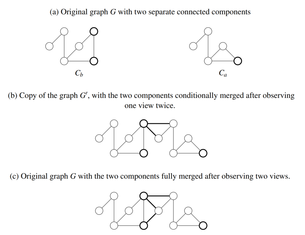
Fig 9: **Conditional merge**. Let us say we require observing one view for a conditional acceptance of a hypothesis, and two views for full acceptance. Part (a) shows a SLAM graph G consisting of two connected components: *C_a*, corresponding to the current new component and *C_b* corresponding to a previously existing component. The view nodes are shown as thick circles. Part (b) illustrates a conditional acceptance after the robot observes one view in *C_b* twice. It shows G’, the copy of G, with two added observation edges from the conditionally accepted hypothesis (thick lines). Part (c) illustrates a full acceptance after observing two views in *C_b*. It shows the new observation edges added to the original graph G.

This is easier said than done, because once two SLAM graph components $C_a$ and $C_b$ are joined, they cannot be easily untangled. The merged graph will be optimized as a whole, affecting the poses of the robot, the views, the occupancy map, and other entities associated with its nodes. Even if we were to keep track of the new edges used to join the connected components, simply removing them would not bring $C_a$ and $C_b$ to their original state.

To get around this problem, we make a copy of the entire SLAM graph. Let $G$ be the SLAM graph, where $C_a \subset G$ and $C_b \subset G$ (Fig. 9a). If we have a merge hypothesis $h_c$ , which is conditionally accepted, then we create $G'$ , which is a copy of $G$ , and where $C'_a$ and $C'_b$ are copies of $C_a$ and $C_b$ respectively. We add the edges from $h_c$ into $G'$ , joining $C'_a$ and $C'_b$ (Fig. 9b). Now, we will use $G'$ for read-only operations, such as looking up the robot pose, or path planning, making the robot behave as though it is localized in the map $C_b$ . However, we still perform all the write operations, such as adding new nodes and edges, and optimization on G, to keep $C_a$ and $C_b$ consistent with their respective original states. Every time $G$ is modified, we copy it into $G'$ and add the edges from $h_c$ , merging $C'_a$ with $C'_b$ .

To fully accept $h_c$ , we simply add the edges corresponding to its observations to $G$ (Fig. 9c). On the other hand, to undo a conditional merge, all we have to do is stop adding the edges from $h_c$ to $G'$ . If there are multiple merge hypotheses present, only one merge hypothesis is allowed to be in a conditionally merged state.

4.3 Preventing Incorrect Recovery

We present an ambiguous view detector on top of the hypothesis filter to help prevent accepting poor recovery hypotheses. A view is defined as ambiguous if in a robot run, that particular view is observable from multiple distinct locations in
an environment leading to rejected observations from the SLAM back-end, while at the same time the robot is certain about its positional estimate w.r.t a recently accepted “trusted” view observation. For a given view $V_y$ , view $V_x$ is “trusted” if $V_x$ was created in the system before $V_y$ . Views marked as ambiguous are discounted in the recovery hypothesis filter. These views can also be discounted from the merge hypothesis filter. Fig. 10 shows an example of ambiguous views and map corruption due to bad recovery hypothesis acceptance.

Fig 10: **Ambiguous views** (a) The bottom of a bed frame looks the same viewed from opposite sides (top image – view from one side, bottom image – view from another side, points and lines – represents matches by our detector). (b) These ambiguous views can cause erroneous edges to be added to the pose graph. Addition of an erroneous edge in this case made the occupancy map become very bad: occupancy cells within the red boundary is duplicated space which is not there.

The ambiguity tracker (Fig.11) contains two observation distance trackers – a rejected view observation distance tracker, and an accepted view observation distance tracker. The distance tracker (DT) keeps track of the distance the robot has traversed since a particular observation was made. Observations in the tracker that exceed a particular distance threshold are removed. Accepted observations go into the accepted observation DT, and rejected observations go into the rejected observation DT.

The rejected observation DT updates a structure V containing views with their number of rejected observations and distance since the first observation periodically. For all views present in V, a check is performed with a preset threshold criteria based on the number of rejected observations and distance since the 1st observation to filter out ambiguous view candidates. The more the number of rejected observations for a particular view, the more the chances of that view being ambiguous.

For all ambiguous view candidates, a second check is performed to determine if they are ambiguous views. This is done with the aid of the accepted observation distance tracker which provides information about “trustworthy” (as defined earlier) views to ascertain positional certainty of the robot. The accepted view distance tracker is used to keep track of recent observations of trustworthy views.

Once a view is determined to be ambiguous, it is marked as such so that it is discounted in the recovery / merge hypothesis filter.

4.4 Erroneous Protrusion Detection

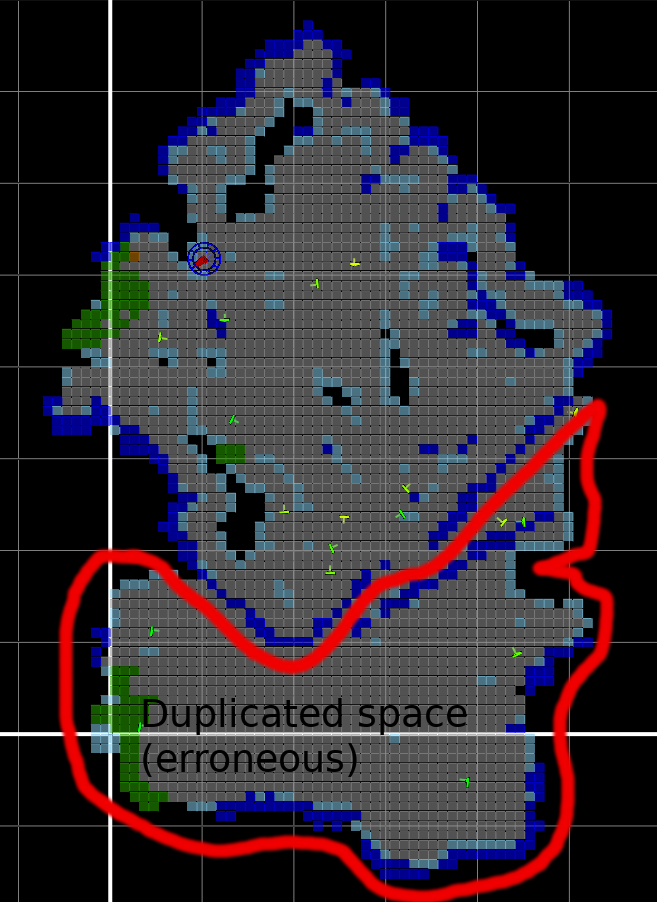
We present a detection mechanism for erroneous protrusions caused due to a failure to detect slip / stasis in a robot. This detector works in the occupancy grid map space.

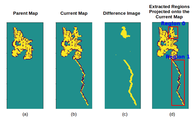
Fig 12: **Erroneous Protrusion Detection**. (a) Initial version of the map. (b) Updated map after run, with new space and protrusion. (c) Image difference between map (a) and (b) detects newly added areas. (d) Classifier detects region 0 as new space and region 1 as erroneous protrusion.

The detector compares a snapshot of the map at the start of a robot’s run (parent map), and a snapshot of the map at present time (current/child map) by performing an image difference operation to segment out the “new” space. The segments are labeled, and run through an erroneous protrusion classifier to determine whether the segment is actually new space discovered in the environment, or an erroneous protrusion (Fig.11). Detected protrusions can be removed from a map, or the map forgotten and the robot can go back to using the parent map.

Feature Selection, Training and Classification: Training data consisting of a mix of parent and child maps with new regions and erroneous protrusions are collected. Regions are segmented and labeled as new regions or protrusions. A set of geometric features such as the average distance transform, bounding box area, area of region, major axis length, minor axis length, and perimeter are computed for each segmented region. For feature selection, ANOVA F-values and their corresponding p-values are computed for all of the features; individual features are looked at as independent variables and can also be augmented with other feature variables. Features with p-values less than 0.05 are selected. Classic machine learning methods such as decision trees, random forests, or support vector machines (SVM) can be used. This classifier can be trained offline, and updated as needed.

4.5 Experiments and Results

4.5.1 Data Set

We used the dataset from Section 3.4.1, i.e. Dataset A, which consists of 965,561 robot runs from 10,000 robots, for evaluating map quality using the metrics described below. A dataset (Dataset B) of 10,000 robot runs in different household environments, and another dataset (Dataset C) consisting of 500,000 maps was used for the evaluation of recovery hypotheses, merge hypotheses, conditional merges, and erroneous protrusion detection.

4.5.2 Map Quality Metrics

The goal here is to keep the map accurate and preserve it’s usefulness to the robot. One indication of the maps usefulness is the stability of the semantic layer over time. We measure that by computing total number of walls in the map, total wall length (perimeter (m)), total map area (m²), and the number of rooms (Fig. 13). We use the consistency of these metrics to determine the success of transferring the semantic information from one run to the next.

Other map quality metrics can be divided into the ones measuring the robot’s ability to relocalize in the map vs. its ability to correct errors in its pose estimate. We measure the former using the relocalization distance, i.e. the distance the robot has to travel before it is able to localize into the map. In this case the distance is a proxy for time, to eliminate the variations in robot’s speed. We measure the latter by devising metrics for how often the robot observes existing views in the map. We calculate the number of view observations per unit area, and the average distance the robot travels between observations.

There are circumstances where the quality of the map is poor and is not captured by any of the aforementioned metrics which might lead to the robot having trouble completing runs, or the user of a robot seeing a mischaracterized environment representation in the semantic map. In these cases, the user might intervene to delete the map and go back to an older map version, or start afresh with the creation of a new map. A map version is defined as the state of the map at the completion of a robot run. Since a map might have been fine for a while before becoming corrupt, we look at the number of times a map version has been deleted. We also look at the number of robots that have had at least one deleted map version.

4.5.3 Evaluation

Fig. 13 shows that the quality of the maps remains good. Semantic map transfer has a very low failure rate, less than 1%, indicating that local occupancy map pruning maintains the overall occupancy map quality.

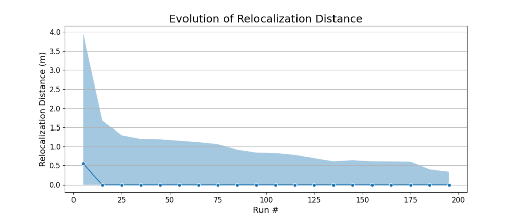
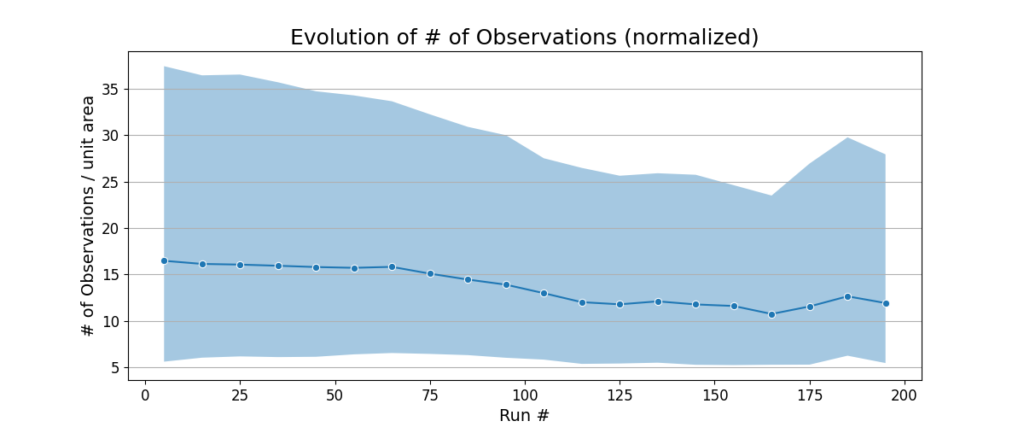
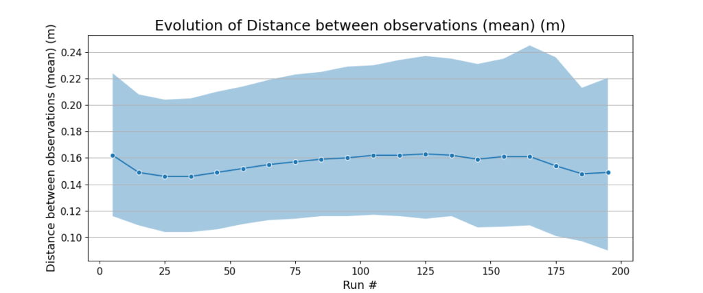
Fig 13: Evolution of map quality over 200 missions in 10k robots. The failure of the semantic map transfer stays below 1%. The relocalization distance, a measure of how fast the robot can relocalize in the map stays low. The number of view observations and the distance traveled between them, indicating the robot’s ability to correct its pose estimates is also stable over time.

The relocalization distance goes down with increasing run number, meaning that the robot is able to relocalize quickly. The number of observations per unit area and distance between observations per unit area stay almost the same across the 200 runs. These metrics indicate that the view management algorithm is able to delete the views that are redundant or unnecessary, while keeping the ones that are useful and observable under a variety of conditions.

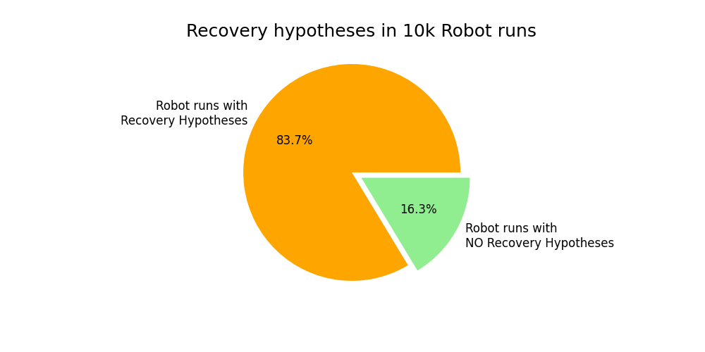
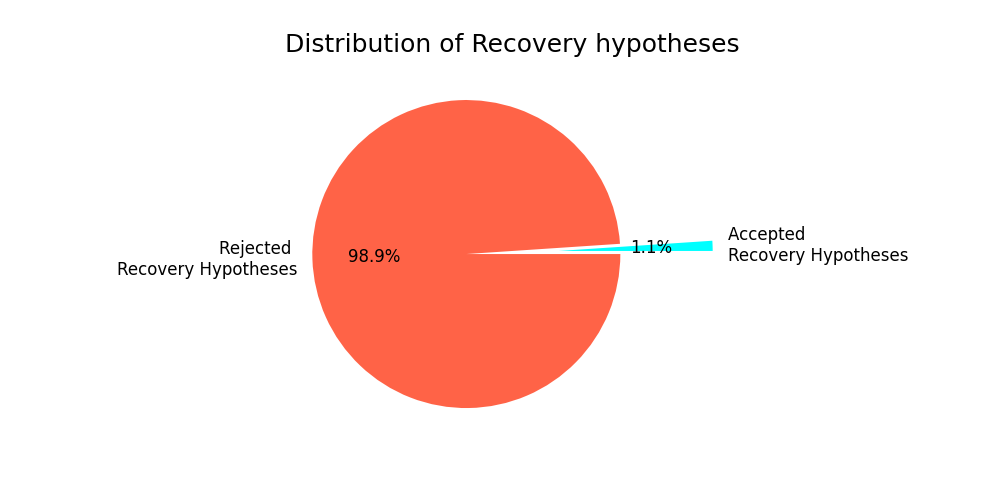
Fig 14: **Recovery hypotheses statistics**. Most robot runs contain recovery hypotheses, but the vast majority is rejected.

Fig. 14 shows the number of recovery hypotheses generated and their acceptance/rejection percentages in Dataset B. We have seen that in a vast majority of the runs, there has been at least one recovery hypothesis created – 83.7%. Out of all the runs with recovery hypotheses, only 1.1% of runs have an accepted recovery hypothesis.

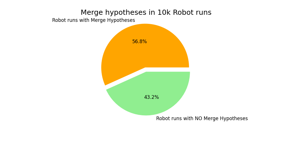
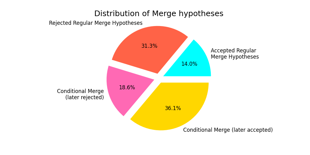
Fig 15: **Merge hypotheses statistics**. In the majority of runs the robot had to relocalize in the map. 18.6% of the merge hypotheses were conditionally accepted and later rejected, preventing possible map corruption.

Fig. 15 shows the number of merge hypotheses generated and their distributions in Dataset B. The robot started localized in a map 43.2% of the time, and the robot had to relocalize (because of a kidnap / reboot) 56.8% of the time. 18.6% of
merges were accepted conditionally, and then rejected later, preventing potential poor relocalizations.

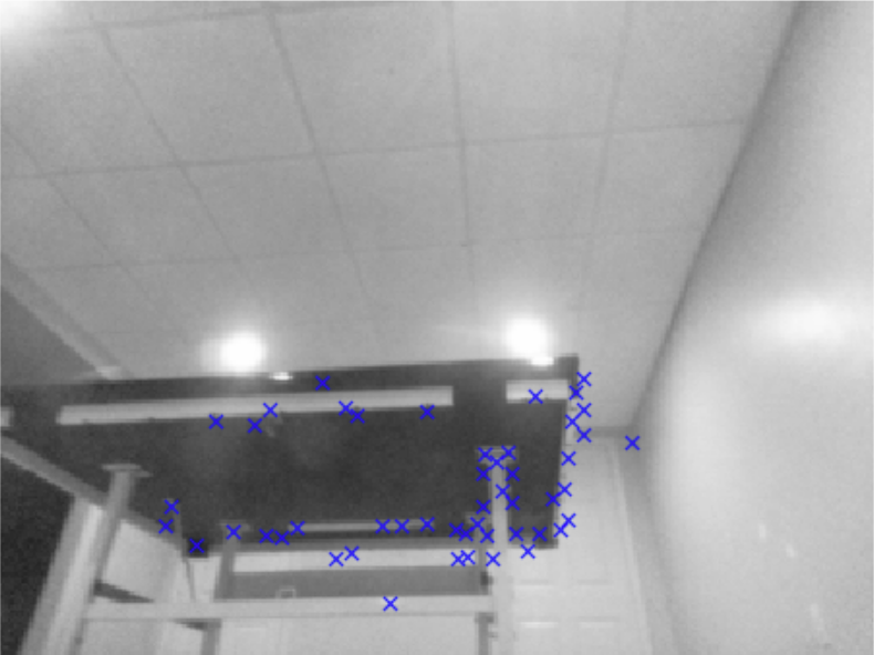
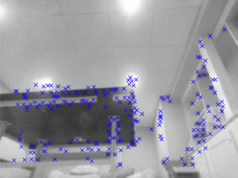
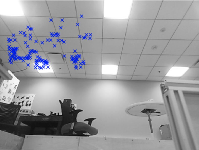
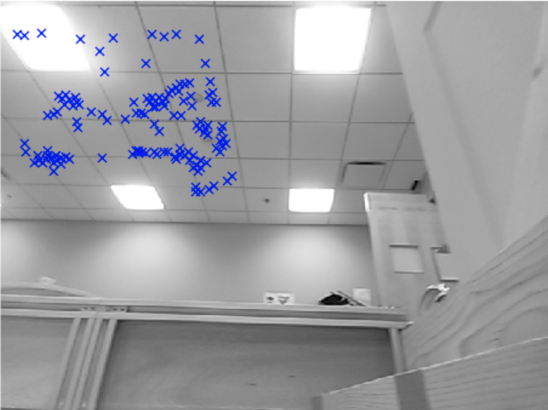
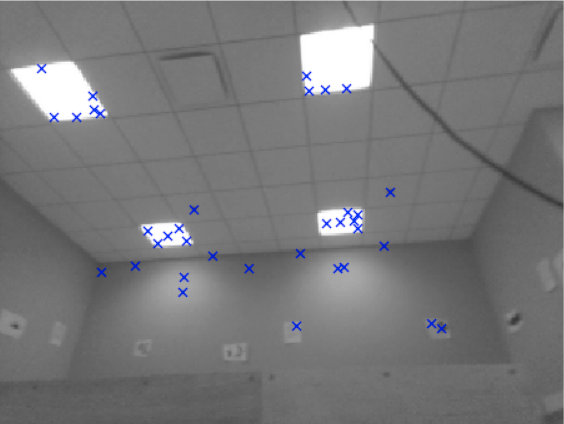
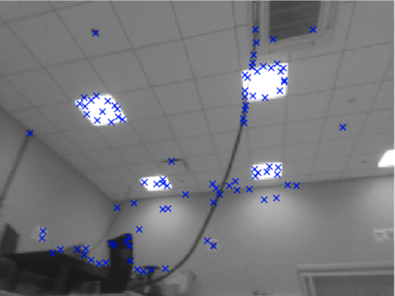
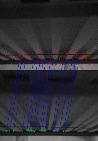
Fig 16: **Ambiguous views**. The ping pong table looks the same viewed from opposite sides. (a) is the view and (b) is an observation. This ambiguous view (a) was detected by our ambiguity tracker and marked as ambiguous.

Fig 17: **Ambiguous views**. The office ceilings look very similar viewed from opposite sides. (a) denote the views and (b) denote observations. These ambiguous views (a) were detected by our ambiguity tracker and were marked as ambiguous.

For ambiguous view detection, our ambiguity tracker parameters were tuned based on a sampling of robot runs with both good and bad accepted recovery hypotheses. The ambiguity tracker was run on a handful of real world samples containing ambiguous views that we had collected – bottom of the bed frame (Fig. 10), ping pong table (Fig. 16), and office ceilings (Fig. 17). We saw a remarkable drop in corrupted maps from those environments using the ambiguity tracker.

Fig 18: **Ambiguous views statistics**. A vast majority of maps contain ambiguous views. The typical number of views per map is about 15-18%.

Fig 19: **Map corruption prevention using ambiguity tracker**. (a) Occupancy map with an erroneous protrusion at the bottom without our ambiguity tracker, caused by adding edges resulting from erroneous observations. (b) With our ambiguity tracker, view from Fig. 16.a was marked as ambiguous and the occupancy map corruption was prevented.

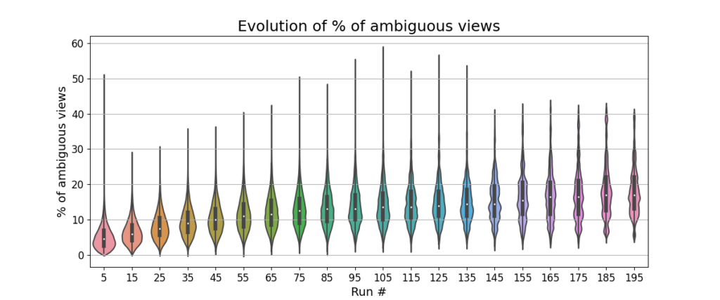
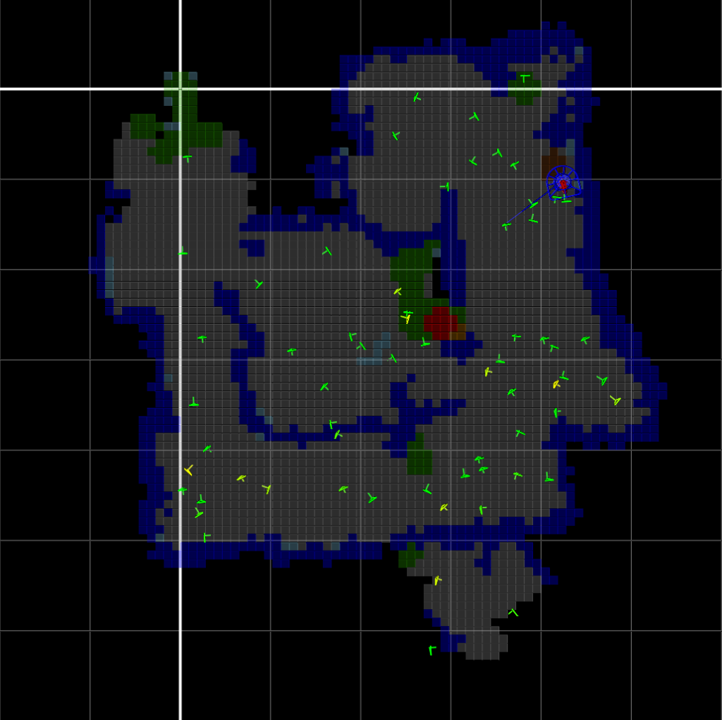
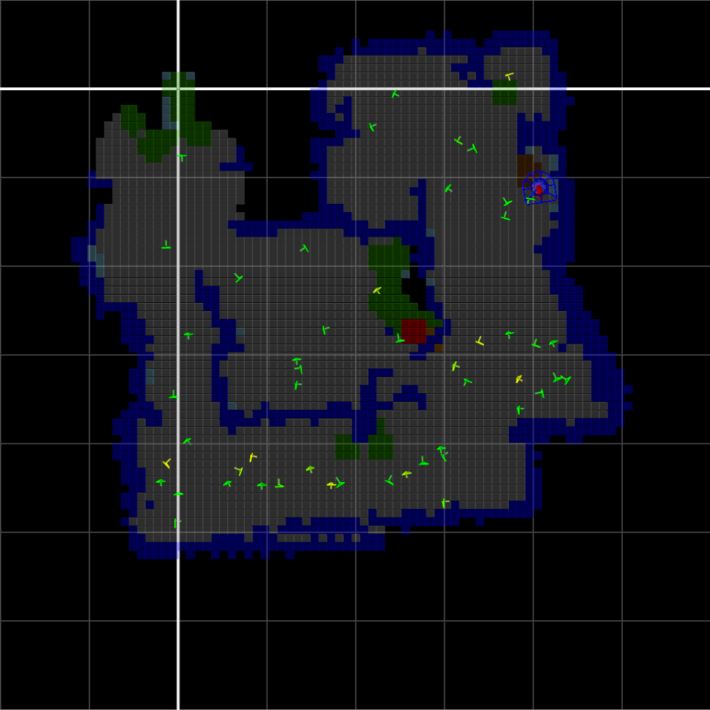
Fig. 16 shows ambiguous views detected by our ambiguity tracker, and Fig. 19 shows a map corruption prevention due to a rejected bad recovery hypothesis because of additional ambiguous view information.

We analyzed ambiguous view detection in Dataset C. Fig. 18 (left) shows that there were almost 90.7% maps containing ambiguous views. Over multiple runs the total number of ambiguous views per map hovers around 15%-18% (Fig. 18
(right)).

In our system, we used a decision tree classifier using the average distance transform, area, and minor axis length features to classify protrusions/new space.

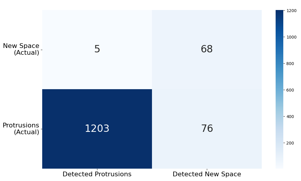
Fig 20: **Erroneous Protrusion Detector confusion matrix**. We have evaluated our method on 1352 maps, where erroneous protrusions and actual newly discovered space were hand-labeled.

Out of 500,000 maps, the erroneous protrusion detector found abnormal protrusions in 4200 maps, or 0.92%. A sampling of 1352 maps containing detected protrusions (1208) and detected new space (144) was user labeled and compared. The confusion matrix (Fig. 20) shows the recall of protrusion detection was 94.05%, and the precision for protrusion detection was 99.58%, with a false positive rate of 0.42%.

Of all the 965,561 map versions corresponding to every single robot run in Dataset A, 3.76% of the map versions were deleted. Of the 10,000 robots, 27.5% of robots had at least one map version that was deleted.

5. Conclusions

We have demonstrated the design, implementation, and deployment of a lifelong mapping system which solves both the complexity issues endemic to local mapping methods and the instability problem for global semantic features. We have evaluated our system with a data set of 10,000 robots in the field and shown that map size, semantic precision, and relocalization performance remain stable and retain their quality over hundreds of missions. We have also described two techniques for preventing map corruption: ambiguous view detection and conditional localization. We also described a method for potentially correcting mistakes in the map after fact by detecting protrusions in the occupancy grid. We demonstrated the efficacy of these methods in keeping the maps usable in lifelong mapping scenarios. The architecture and algorithms our system uses to achieve lifelong mapping are modular and can be adapted to meet a broad class of SLAM powered robots in the wild.

6. Acknowledgments

This work was done at iRobot. This work would not have been possible without the work and support of the mehcanical, electrical, and the software engineering teams at iRobot. This work was done over a considerable period of time with the input of various engineers who are experts in SLAM, computer vision, and other related disciplines. Some of those engineers are co-authors on the published articles.

Nandan Banerjee